Load, Save, and .rda files

A couple weeks ago I stumbled across a feature in R that I had never heard of before. The functions save(), load(), and the R file type .rda.

The .rda files allow a user to save their R data structures such as vectors, matrices, and data frames. The file is automatically compressed, with user options for additional compression. Let’s take a look.

First, we will grab one of the built-in R datasets. We can view these by calling data(). Let’s use the “Orange” dataset.

# get the Orange data
Orange
   Tree  age circumference
1     1  118            30
2     1  484            58
3     1  664            87
4     1 1004           115
5     1 1231           120
6     1 1372           142
7     1 1582           145
8     2  118            33
9     2  484            69
10    2  664           111
11    2 1004           156
12    2 1231           172
13    2 1372           203
14    2 1582           203
15    3  118            30
16    3  484            51
17    3  664            75
18    3 1004           108
19    3 1231           115
20    3 1372           139
21    3 1582           140
22    4  118            32
23    4  484            62
24    4  664           112
25    4 1004           167
26    4 1231           179
27    4 1372           209
28    4 1582           214
29    5  118            30
30    5  484            49
31    5  664            81
32    5 1004           125
33    5 1231           142
34    5 1372           174
35    5 1582           177

Next, let’s save each column individually as vectors.

# save the Orange data as vectors
count<-Orange$Tree
age<-Orange$age
circumference<-Orange$circumference

Now if we look at our variables in the RStudio environment, we can see count, age, and circumference saved there.

Next, let’s set our R working directory, so the .rda file will save in the correct location. First we’ll use getwd() to find our current working directory, then we’ll adjust it (if needed) using setwd(). I set my working directory to a folder on the D drive.

#get and set working directory
getwd()
[1] "D:/Users"
setwd("D:/r-temp")
> getwd()
[1] "D:/r-temp"

Finally, let’s use the save() command to save our 3 vectors to an .rda file. The “file” name will be the name of the new .rda file.

#save to rda file
save(count, age, circumference, file = "mydata.rda")

Next we will remove our R environment variables using the command rm().

#remove variables
rm(age, circumference, count)

Now we can see that we no longer have saved variables in our R workspace.

Now, we can check that our .rda file (myrda.rda) does in fact store our data by using the load() command.
Note: If we had not properly set our working directory, then we would have needed to provide a full path to the rda file. For example, “C:/Users/Documents/R files/myrda” rather than just “myrda”.

#load the rda file
load(file = "mydata.rda")

Great, now we can see that our variables are back in the R environment for use once more.

Saving and loading data in R might be very useful when you’re working with large datasets that you want to clear from your memory, but you also would like to save for later. It also might be useful for long, complex R workflows and scripts. You can control the compression of the file using the settings ‘compress’ and ‘compression_level’.

That’s all for now!

Importing Data into R, part II

I recently downloaded the latest version of R Studio and noticed that their import dataset functionality had changed significantly. I had previously written about importing data HERE and wanted to provide an update for the current version of RStudio.

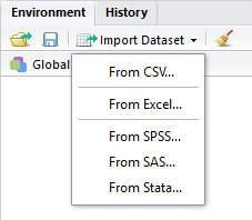
When you go to import data using R Studio, you get a menu like this.

If you’re using the latest version of RStudio, when you click “From CSV” you’ll get a popup about downloading a new library ‘readr’.

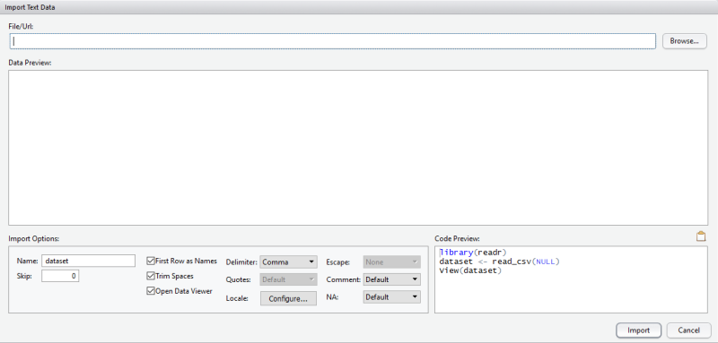
Once that has completed, you’ll see the new import data window (shown below).

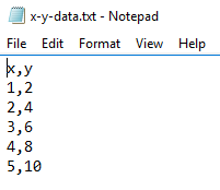
Okay, so first let’s make a simple comma delimited data file so we can test out the new import dataset process. I have made a simple file called “x-y-data.txt” as shown below. If you make this same file (no spaces, just a comma to separate the x column from the y column) then we can do this exercise together.

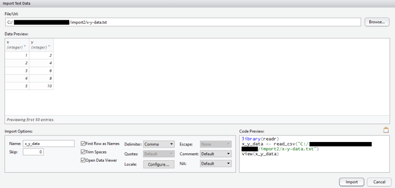
Now, let’s use the RStudio import to bring in the file “x-y-data.txt”. Here’s a screen grab of the import screen with my x-y dataset.

We can see that RStudio has used the first row as names, has recognized that it is a comma delimited file, and has read both x and y values as integers. Everything looks good, so I click “import”.

It was after this import process, that I had tried running some of my standard functions, such as making an empirical CDF (cumulative density function) and then I ran into problems. So let’s check the type of data we have imported.

# get the data structure
typeof(x_y_data)
#[1] "list"
class(x_y_data)
#[1] "tbl_df"     "tbl"        "data.frame"

While the old RStudio would have imported this as a matrix by default, this latest version of RStudio imports data as a data frame by default. Apparently RStudio has created their own version of a data frame called a “tbl_df” or tibble data frame. When you use the ‘readr’ package, your data is imported automatically as a “tbl_df”.

Now this isn’t necessarily a bad thing, in fact it seems like there is some nice functionality gained by using the “tbl_df” format. This change just broke some of my previously written code and it’s good to know what RStudio is doing by default.

If we wanted to get back to the matrix format, we can do this will a simple as.matrix function. From there we can verify it was converted using the typeof and class functions.

# convert to a matrix
data<-as.matrix(x_y_data)
#     x  y
#[1,] 1  2
#[2,] 2  4
#[3,] 3  6
#[4,] 4  8
#[5,] 5 10

typeof(data)
#[1] "integer"
class(data)
#[1] "matrix"

You can read more about the new Tibble structure at these websites:

https://blog.rstudio.org/2016/03/24/tibble-1-0-0/

http://www.sthda.com/english/wiki/tibble-data-format-in-r-best-and-modern-way-to-work-with-your-data

Enjoy!

Secret Santa Picker 2 using R

Last year I made a blog post about a Secret Santa picker HERE, but to use it required quite a bit of messing around with the code. So this year I decided to improve the whole thing by making it a function rather than a script. The function take two inputs, a list of names and a number of names. The code for the function is listed first followed by the code for the script used to call the function.

Here’s the function. Nothing needs to be changed in this code for it to run properly.

# make a function 
secret_santa <-function(npeople, names){
  
  # this 'flag' is used to determine if the
  # function stays in or out of the while function
  flag = "bad"
  
  # first list of names
  namelist1 = matrix(names, ncol = 1, nrow = npeople)
  fam = matrix(ncol = 1, nrow = npeople, NA)
  
  while (flag == "bad"){
    
    # names to choose from
    namelist2 = matrix(ncol = 1, nrow = npeople, NA)
    
    for (i in 1:npeople){
      #pick the first name
      if (i==1){
        xx2 = sample(names, (npeople-i+1), replace=FALSE)
      } else
        xx2 = sample(xx2, (npeople-i+1), replace=FALSE)
      
      if (i == npeople & xx2[1]==namelist1[i,1]){
        flag = "bad"
        
      }else if(xx2[1]!= namelist1[i,1]){
        namelist2[i,1] = xx2[1]
        flag = "good"
      } else{
        namelist2[i,1] = xx2[2]
        flag = "good"
        }
      
      
      #set up the new matrix with one less name
      used = which(xx2==namelist2[i])
      xx2[used] = "zzzzz"
      xx2 = sort(xx2)[1:(npeople-i)]
    }
    
    #flag
    #add "has" to the matrix
    has = matrix(ncol=1, nrow = npeople, "has")
    
    #build the final matrices
    final = cbind(namelist1, has, namelist2)	
    #the final results
    #final
    
    
  }
  final
}

Save this function as “secret-santa-function.R” and we’ll call it from our script. Okay, now let’s make our script.

# call the function from the script
source("secret-santa-function.R")

### Function input
### make a list of names
names = c("James","Nick","Emily","Natasha","Bob", "Teddy")
n = length(names)

#call the function
output <-secret_santa(n, names)
output 

The list of names is the only input needed. In the case above it’s ‘names = c(“James”,”Nick”,”Emily”,”Natasha”,”Bob”, “Teddy”)’. The other variable the function needs is the number of names, which is read automatically from the length function. That’s it, you’re done. Call the function from the script and you’ve got your names.

Make a bar plot with ggplot

The first time I made a bar plot (column plot) with ggplot (ggplot2), I found the process was a lot harder than I wanted it to be. This post steps through building a bar plot from start to finish.

First, let’s make some data. I’m going to make a vector of months, a vector of the number of chickens and a vector of the number of eggs. That’s random enough for this purpose.

# make some data
months <-rep(c("jan", "feb", "mar", "apr", "may", "jun", 
               "jul", "aug", "sep", "oct", "nov", "dec"), 2)
chickens <-c(1, 2, 3, 3, 3, 4, 5, 4, 3, 4, 2, 2)
eggs <-c(0, 8, 10, 13, 16, 20, 25, 20, 18, 16, 10, 8)
values <-c(chickens, eggs)
type <-c(rep("chickens", 12), rep("eggs", 12))
mydata <-data.frame(months, values, type)

If parts of the above code don’t make sense, take a look at my post on using the R functions seq (sequence), rep (repeat), and cbind (column bind) HERE.

Now let’s load the ggplot package.

library(ggplot2)

We want to make a plot with the months as the x-axis and the number of chickens and eggs as the height of the bar. To do this, we need to make sure we specify stat = “identity”. Here’s the basic code for this plot.

p <-ggplot(mydata, aes(months, values))
p +geom_bar()

Notice that you will get the error shown above, “stat_count() must not be used with a y aesthetic.” We forgot to specify that we want the height of the column to equal the value for that month. So let’s do it again.

p <-ggplot(mydata, aes(months, values))
p +geom_bar(stat = "identity")

This time we get a plot, but it looks fairly ugly, and the months are out of order. In fact the months are in alphabetical order so let’s fix that first. If we investigate the months, we will see they have ordered levels.

mydata$months
#[1] jan feb mar apr may jun jul aug sep oct nov dec jan feb mar apr may
#[18] jun jul aug sep oct nov dec
#Levels: apr aug dec feb jan jul jun mar may nov oct sep

We can fix the order of this category by changing the factor. Here’s some code that will fix our problem.

mydata$months <-factor(mydata$months, 
                      levels = c("jan", "feb", "mar", "apr", "may", "jun",
                                 "jul", "aug", "sep", "oct", "nov", "dec"))

Now if we look at the levels again, we will see that they’re rearranged in the order that we want.

mydata$months
#[1] jan feb mar apr may jun jul aug sep oct nov dec jan feb mar apr may
#[18] jun jul aug sep oct nov dec
#Levels: jan feb mar apr may jun jul aug sep oct nov dec

Okay, let’s make our plot again, this time with the months in the correct order.

p <-ggplot(mydata, aes(months, values))
p +geom_bar(stat = "identity", aes(fill = type)) 

Okay, now the months are working, but we realize we only have one set of columns being plotted. We should have two sets, ‘chickens’ and ‘eggs’. To fix this we need to specify some feature that separates them. We already created this in the “type” column when we made our data frame.

If we make the color of the graphs based off of the data category then we should get two sets of columns. In our data frame, we put our categories in the column named “type”. Fill is a property of bar plots. If we were making a line plot and we wanted to set the colors by the type of data we would use color = type rather than fill = type.

p <-ggplot(mydata, aes(months, values))
p +geom_bar(stat = "identity", aes(fill = type))

Cool! Sort of. We have stacked bar plots, but I want them next to one another, not stacked. We can fix that with one more change to our code using dodge.

p <-ggplot(mydata, aes(months, values))
p +geom_bar(stat = "identity", aes(fill = type), position = "dodge")

Finally, let’s spruce the plot up a little bit. We’ll adjust the x-axis label (xlab), y-axis label (ylab), title (ggtitle) and update the look using theme_bw().

p <-ggplot(mydata, aes(months, values))
p +geom_bar(stat = "identity", aes(fill = type), position = "dodge") +
  xlab("Months") + ylab("Count") +
  ggtitle("Chickens & Eggs") +
  theme_bw()

The plot finally looks good and we’re done. Happy plotting!

Importing Data into R

One of the most important features we need to be able to do in R is import existing data, whether it be .txt files, .csv files, or even .xls (Excel files). If we can’t import data into R, then we can’t do anything. Okay let’s get started.

The spirit of this blog is that whatever I do here, should also work for someone working from home. Thus, we all need to work from the same text file, so we have to build a simple text file together to make this whole process work. Since this isn’t R code, I’ll just break it down into simple steps that are easy to follow.

Step 1: open notepad
Step 2: enter data as I have shown below (no spaces, use only commas)

Step 3: save the file as ‘rain.txt’ on your Desktop

Okay, great now it’s time to get to work in R importing this data. We have two options, importing using the R Studio environment (the easy way), or importing using standard R functions.

The Easy way (Import through R Studio)

Step 1: Click the ‘Import Dataset’ button, then click ‘From Local File’

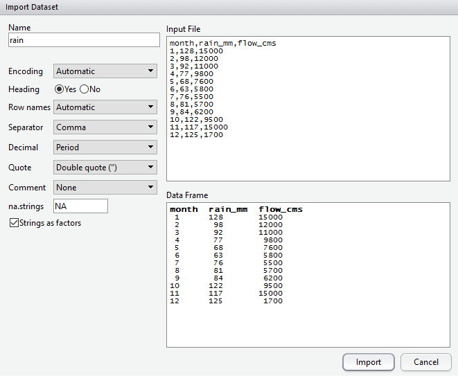
Step 2: Navigate to the ‘rain.txt’ file located on your Desktop and click ‘open’. The next dialog box we get shows the values contained within our file, and different importing options. A few things to notice, ‘Name’ at the top has been set to “rain”, which will become the variable our data is stored as in R. The ‘Heading’ radio button has already been moved to ‘yes’ because R Studio has recognized our column headers (month, rain_mm, flow_cms). Additionally, the ‘Separator’ has been adjusted to ‘comma’ as we have made a comma delimited text file. All you have to do is just click ‘Import’.

Step 3: R Studio automatically opens the ‘rain’ dataset as a table in a new tab. R Studio also provides the snippet of code it used to import the data, which is great! You can copy that code and paste it into your R script file for future use.

That’s it! You’re a pro at importing data using R Studio.

 The Hard way (Import using R functions)

There’s lots of functions that can be used to import data into R: read.table, read.csv, read.csv2, read.delim, read.delim2 (among others). We’ll use read.table in this example.

To understand how this function works, let’s open up the R help by typing ?read.table.

# Get R help
?read.table

That should open up a help file through your web browser, or in the lower right ‘Help’ menu if you’re using R Studio. The main pieces of this function we need to set are ‘file’, ‘header’, and ‘sep’.
-The ‘file’ piece is the file name and file path we want to import.
-The ‘header’ piece is set to TRUE or FALSE based on whether or not there is a header within the file.
-The ‘sep’ piece describes the separator used within the file (in our case, a comma)

So, here’s how our code should look:

# Import the data
rain<-read.table("C:/Users/YOUR-NAME/Desktop/rain.txt", header = TRUE,
                   sep = ",")

Two things of note in the code above.
-The part of the path “YOUR-NAME” is based on your computer login settings. It might be something like ‘Tim’, ‘Jane’, ‘PeterC’, etc.
-I have defined this data as “rain” in R, using the rain <- bit of code. Here’s how the data looks in R.

# The rain data
#   month rain_mm flow_cms
#1      1     128    15000
#2      2      98    12000
#3      3      92    11000
#4      4      77     9800
#5      5      68     7600
#6      6      63     5800
#7      7      76     5500
#8      8      81     5700
#9      9      84     6200
#10    10     122     9500
#11    11     117    15000
#12    12     125     1700

That’s it! You’re a pro at importing data into R via the hard way! Happy coding!

 

2 y-axis plotting

A simple plotting feature we need to be able to do with R is make a 2 y-axis plot. First let’s grab some data using the built-in beaver1 and beaver2 datasets within R. Go ahead and take a look at the data by typing it into R as I have below.

# Get the beaver datasets
beaver1
beaver2

We’re going to plot the temperatures within both of these datasets, which we can see (after punching into R) is the third column.

First let’s check the length of these datasets and make sure they’re the same.

# Get the length of column 3
length(beaver1[,3])
length(beaver2[,3])

[1] 114
[2] 100

Since beaver1 is longer, we’ll only plot rows 1 through 100 of the temperature data, so that it is the same length as beaver2.

# Plot the data
plot(beaver1[1:100, 3], type ="l", ylab = "beaver1 temperature")

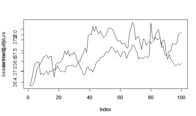
Cool, your plot should look like this.

Now, let’s add that second dataset on the right y-axis. So, we have to have to create a plot on top of this plot using the command par(new = TRUE).

# Add the second y-axis
plot(beaver1[1:100, 3], type ="l", ylab = "beaver1 temperature")
par(new = TRUE)
plot(beaver2[,3], type = "l")

Woah, this plot is ugly! We have 2 y-axis labels plotting, 2 y-axis values plotting, and 2 x-axis values and labels plotting. Let’s turn those off using the commands xaxt = “n” and yaxt = “n”.

# updated plot
plot(beaver1[1:100, 3], type ="l", ylab = "beaver1 temperature")
par(new = TRUE)
plot(beaver2[,3], type = "l", xaxt = "n", yaxt = "n",
     ylab = "", xlab = "")

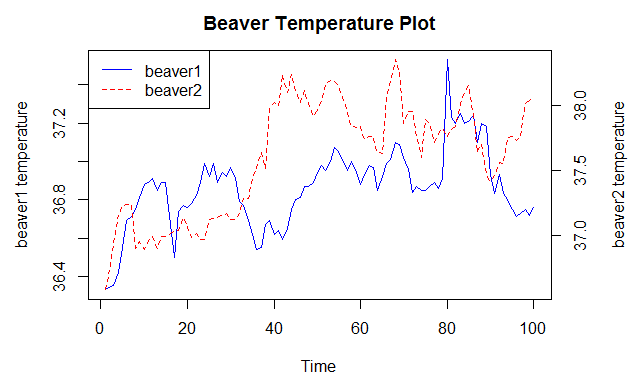
Okay, it’s still pretty ugly, so let’s clean it up. Let’s make the margins bigger on the right side of the plot, add a y2 axis label, add a title, change the color of the lines and adjust the x-axis label. Don’t forget the legend! Here’s the code:

# final plot
par(mar = c(5, 5, 3, 5))
plot(beaver1[1:100, 3], type ="l", ylab = "beaver1 temperature",
     main = "Beaver Temperature Plot", xlab = "Time",
     col = "blue")
par(new = TRUE)
plot(beaver2[,3], type = "l", xaxt = "n", yaxt = "n",
     ylab = "", xlab = "", col = "red", lty = 2)
axis(side = 4)
mtext("beaver2 temperature", side = 4, line = 3)
legend("topleft", c("beaver1", "beaver2"),
       col = c("blue", "red"), lty = c(1, 2))

Woo! Looks good. That’s all for now.

ggplot2 (ggplot) Introduction

In this post I’ll briefly introduce how to use ggplot2 (ggplot), which by default makes nicer looking plots than the standard R plotting functions.

The first thing to know is that ggplot requires data frames work properly. It is an entirely different framework from the standard plotting functions in R. Let’s grab a default data frame in R called mtcars. Let’s confirm it’s a data frame using some code:

# Get the mtcars data types
class(mtcars)

R confirms that this is in fact a data frame.

# the output
[1] "data.frame"

Feel free to take a look at the data itself by just typing the name into R. For bevity, I won’t show the data in this post.

# Look at mtcars
mtcars

Next let’s define some standard plot function names in ggplot.
geom_point = scatterplot (points or solid lines)
geom_boxplot = boxplot
geom_bar = column plot
There’s many more (really cool) plot types, but I’ll stop here for now.

Let’s make our scatterplot. Here’s the code to make a standard plot. Don’t forget to load the package ggplot2 before running this code using the library function (install ggplot2 first if you haven’t done so before).

# Plot the data
library(ggplot2)
ggplot(mtcars, aes(hp, mpg)) + geom_point()

Success! The code above seems strange at first, but let’s dive into how it works. First we call ggplot and provide the data frame name ‘mtcars’. Then we give the x & y variables using the aes command. Finally we specify we’re making a scatterplot by attaching + geom_point().

Now let’s make this look better! This is where the power of ggplot shines. It’s really easy to make a nice looking plot.

# Plot the data
p <- ggplot(mtcars, aes(hp, mpg))
p + geom_point() + labs (x = "Horsepower (hp)", y = "Miles per Gallon (mpg)") +
  ggtitle("My mtcars Plot")

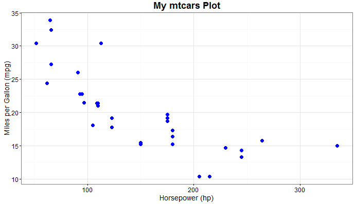
We can see that the syntax is a bit different this time. We save the first ggplot call to a variable p (p for plot), but any variable will work. Then we attached more plotting features using p + ——. For this plot we added custom x and y axis labels and a title.

Next let’s make a change to the overall look of the plot, using what ggplot calls a theme. We’ll add theme_bw.

# Plot the data
p <- ggplot(mtcars, aes(hp, mpg))
p + geom_point() + labs (x = "Horsepower (hp)", y = "Miles per Gallon (mpg)") +
  ggtitle("My mtcars Plot") + theme_bw()

Finally, let’s spruce it up my coloring the points blue and making them bigger, while also making our axes and titles bigger. The code below makes this final plot.

# Make the final plot
p <- ggplot(mtcars, aes(hp, mpg))
p + geom_point(size = 3, color = "blue") + 
  labs (x = "Horsepower (hp)", y = "Miles per Gallon (mpg)") +
  ggtitle("My mtcars Plot") + theme_bw()+
  theme(axis.text = element_text(size = 12), 
        axis.title = element_text(size = 14),
        plot.title = element_text(size = 18, face = "bold"))

Hope this helped explain the basics of ggplot. Here’s the link to the ggplot2 documentation (click me).

Multiplication (and R data types)

This is a basic post about multiplication operations in R. We’re considering element-wise multiplication versus matrix multiplication. First let’s make some data:

# Make some data
a = c(1,2,3)
b = c(2,4,6)
c = cbind(a,b)
x = c(2,2,2)

If we look at the output (c and x), we can see that c is a 3×2 matrix and x is a 1×3 matrix (which I will also call a vector).

# View our data
c
##      a b
## [1,] 1 2
## [2,] 2 4
## [3,] 3 6
x
## [1] 2 2 2

In R the asterisk (*) is used for element-wise multiplication. This is where the elements in the same row are multiplied by one another.

#These will give the same result
c*x
x*c

We can see that the output of c*x and x*c are the same, and the vector x doubles matrix c.

#View our element-wise multiplication output
##      a  b
## [1,] 2  4
## [2,] 4  8
## [3,] 6 12

##      a  b
## [1,] 2  4
## [2,] 4  8
## [3,] 6 12

In R percent signs combined with asterisks are used for matrix multiplication (%*%).

# This works (matrix multiplication)
x%*%c
##       a  b
## [1,] 12 24

If you dig back and remember your matrix multiplication, you’ll find that a 1×3 matrix times a 3×2 matrix gives a 1×2 matrix. It will have the same number of rows as the first matrix (x has 1 row) and the same number of columns as the second matrix (c has 2 columns). Now let’s try this with x and c reversed.

# This doesn't work. Incorrect dimensions.
c%*%x
## Error in c %*% x : non-conformable arguments

R gives us an error because you can’t multiply a 3×2 and 1×3 matrix. For the matrix multiplication to work, the number of columns in the first matrix (c = 3 columns) has to be equal to the number of rows in the second matrix (x= 1 row).

The previous operations were done using the default R arrays, which are matrices. We can confirm this using the command class and typeof below:

# Get the data type
class(c)
typeof(c)
class(x)
typeof(x)

Here’s the output of those functions.

# The output
## [1] "matrix"
## [1] "double"
## [1] "numeric"
## [1] "double"

This shows us that our matrix c, has the R data type of a matrix, with formatting of ‘double’, which means that is is numbers (as opposed to something like ‘character’). This also shows us our 1×3 matrix or vector has the R data type ‘numeric’ and also has the formatting of ‘double’.

Now, let’s say your data is in a data frame rather than a matrix. Let’s see what happens when we perform multiplication on data frames. Remember data frames in R can hold different types of data (numbers, letters, etc.), while matrices can only have one type of data.
***For more info about this see my post here titled CBIND2***
Let’s convert our matrices to data frames using the function data.frame.

c1 = data.frame(c)
x1 = data.frame(x)

Now let’s look at our data. Note that there is an extra column of numbers from 1 to 3 for both c1 and x1. This is just a feature of the data frame output in R, where it is counting the rows 1 through 3.

c1
##   a b
## 1 1 2
## 2 2 4
## 3 3 6

x1
##   x
## 1 2
## 2 2
## 3 2

And just to be thorough, let’s check the R data type, to make sure they are not matrices.

# Check the data type
class(c1)
typeof(c1)
class(x1)
typeof(x1)

Here’s the output of those the data type. Notice that the class is now ‘data.frame’ instead of ‘matrix’ or ‘numeric’.

# The output
## [1] "data.frame"
## [1] "list"
## [1] "data.frame"
## [1] "list"

Now let’s try our simple element-wise multiplication again. You may have guessed it already, but these functions will no longer work.

# These both do not work
c1*x1
x1*c1

Here’s the output of the multiplication (i.e., the errors R provides).

## Error in Ops.data.frame(c1, x1) : 
##   ‘*’ only defined for equally-sized data frames

## Error in Ops.data.frame(c1, x1) : 
##   ‘*’ only defined for equally-sized data frames

According to the error R is providing, we can only multiply data frames of the same size. So, let’s try this out by making some new data.

# Make some data
h=c(2,2)
k=c(4,4)
j=cbind(h,k)
l=j*2

df1 = data.frame(j)
df2 = data.frame(l)

Now let’s look at the data to see what we have

# View the new data frames
df1
##   h k
## 1 2 4
## 2 2 4

df2
##   h k
## 1 4 8
## 2 4 8

Finally, let’s multiply df1*df2 and see what happens.

# Data frame multiplication
df1*df2
##   h  k
## 1 8 32
## 2 8 32

R has done element-wise multiplication on the data frames. This makes sense since we use only the (*) command. If we try this again with the order of the data frames reversed, we will get the same answer.

# Reverse the order for multiplication
df2*df1
##   h  k
## 1 8 32
## 2 8 32

That’s all for now. Hopefully this shed more light onto the way R performs multiplication, especially based on the data type.

How to make a Function in R

This post is meant to show R users how to make their own functions. We’ll start with an easy example below.

Most of my posts provide R code that can be easily copied into R and replicated at home. This post will be a break from that process since functions require saving *.R files and calling them from other *.R files. Let’s begin.

First of all make a new R script file. This will become our function file. There is no difference between a script file and a function file in R. Both are *.R files.

We will make a simple function that multiplies a vector of data by 2. We start by defining our function using the

#make a function
my_function<- function(x){
  x*2
  
}

Now save this R file as “f_myfirstfunction.R” on your Desktop. Now let’s walk through the components of the function. We defined it as “my_function”. This is important as it is how we call the function. After that it’s the

Now we have to open a second R file. This will be the script file that we will use to call the function from. We’ll start this file by setting our working directory to the desktop with the functions getwd() and setwd. getwd() simply states your current working directory in R. setwd is used to change it to wherever you like.

#set the working directory
#rename "your User Name here" based on your user name
#example: owner, Emily, Bill
getwd()
setwd("C:/Users/your User Name here/Desktop")
currwd 

If you get the error, “Error in setwd(“C:/Users/your User Name here/Desktop”):
cannot change the working directory” that means you misspelled some part of your file path. Fix the error and run the code again.

Now we need to make a vector of data, so let’s use the function seq which makes a sequence of values. We’ll save our vector as “data”.

#make some data
data<- seq(from=1, to=10, by=1)
data

Next we have to import the function that we made into the R working space. This is very easy once we have set the working directory. Simply use the call source.

#import the function
source("f_myfirstfunction.R")

I should point out that you need quotations around the R file name. Also, if this file is not saved on the Desktop (the location we set the working directory to), this will give an error “Error in file (….. cannot open the connection”. If this happens move your function file “f_myfirstfunction.R” to your working directory.

Now we will use our awesome new function that we made to multiply the vector “data” by 2. Of course we could just code data*2, but that’s not the point. We’re learning how to write a function.

#call the function
my_function(data)

Awesome! You ran your first function! The R console will spit out the answer:
[1] 2 4 6 8 10 12 14 16 18 20
If we wanted to do something more useful with this output we should save it as a variable. Let’s use data2.

#call the function
data2 <- my_function(data)

This time we get no output from R, but if we type in the variable data2 we get our familiar output:
[1] 2 4 6 8 10 12 14 16 18 20

One important thing to remember when using functions in R is that it doesn’t matter what you save you function file as. When you call your function, you’re using the defined name within the function file code.

#rename the function call to 'times2'
times2<- function(x){
  x*2
}

#rename the function again
zzzzz<- function(x){
  x*2
}

This is the same function saved in file “f_myfirstfunction.R”, but the function name has been changed. Again the function name is what is called from R.

I’ve listed the full text of the script file “call function.R” and the function file “f_myfirstfunction.R” below.

Hope this helps! Happy function writing!

#"call function.R"
#set the working directory
getwd()
setwd("D:/D Documents/wordpress/practicalR/make a function")
currwd

#make some data
data<- seq(from=1, to=10, by=1)
data

#import the function
source("f_myfirstfunction.R")

#call the function
my_function(data)

#call the function - save output as variable
data2 <- my_function(data)
 

#"f_myfirstfunction.R"
my_function<- function(x){
  x*2
}

Secret Santa Picker using R

Here’s a quick post on making a secret santa picker using R. The code eliminates a person from picking themselves, otherwise it’s no frills.

#set the variable for the number of people
npeople=5

fam=matrix(ncol=1, nrow=npeople, NA)
fam[1,1]="name1"
fam[2,1]="name2"
fam[3,1]="name3"
fam[4,1]="name4"
fam[5,1]="name5"


fam2=matrix(ncol=1, nrow=npeople, NA)
names=c("name1","name2","name3","name4","name5")
for (i in 1:npeople){
  #pick the first name
  if (i==1){
    xx2=sample(names, (npeople-i+1), replace=FALSE)
  } else
    xx2=sample(xx2, (npeople-i+1), replace=FALSE)
  
  if (xx2[1]!=fam[i,1]){
    fam2[i,1]=xx2[1]
  } else{
    fam2[i,1]=xx2[2]}
    
  
  #set up the new matrix with one less name
  used=which(xx2==fam2[i])
  xx2[used]="zzzzz"
  xx2=sort(xx2)[1:(npeople-i)]
}

#add "has" to the matrix
has=matrix(ncol=1,nrow=npeople, "has")

#build the final matrices
final=cbind(fam,has,fam2)	
#the final results
final

[,1] [,2] [,3]
[1,] “name1” “has” “name4”
[2,] “name2” “has” “name3”
[3,] “name3” “has” “name5”
[4,] “name4” “has” “name2”
[5,] “name5” “has” “name1”