How to make a Function in R

This post is meant to show R users how to make their own functions. We’ll start with an easy example below.

Most of my posts provide R code that can be easily copied into R and replicated at home. This post will be a break from that process since functions require saving *.R files and calling them from other *.R files. Let’s begin.

First of all make a new R script file. This will become our function file. There is no difference between a script file and a function file in R. Both are *.R files.

We will make a simple function that multiplies a vector of data by 2. We start by defining our function using the

#make a function
my_function<- function(x){
  x*2
  
}

Now save this R file as “f_myfirstfunction.R” on your Desktop. Now let’s walk through the components of the function. We defined it as “my_function”. This is important as it is how we call the function. After that it’s the

Now we have to open a second R file. This will be the script file that we will use to call the function from. We’ll start this file by setting our working directory to the desktop with the functions getwd() and setwd. getwd() simply states your current working directory in R. setwd is used to change it to wherever you like.

#set the working directory
#rename "your User Name here" based on your user name
#example: owner, Emily, Bill
getwd()
setwd("C:/Users/your User Name here/Desktop")
currwd 

If you get the error, “Error in setwd(“C:/Users/your User Name here/Desktop”):
cannot change the working directory” that means you misspelled some part of your file path. Fix the error and run the code again.

Now we need to make a vector of data, so let’s use the function seq which makes a sequence of values. We’ll save our vector as “data”.

#make some data
data<- seq(from=1, to=10, by=1)
data

Next we have to import the function that we made into the R working space. This is very easy once we have set the working directory. Simply use the call source.

#import the function
source("f_myfirstfunction.R")

I should point out that you need quotations around the R file name. Also, if this file is not saved on the Desktop (the location we set the working directory to), this will give an error “Error in file (….. cannot open the connection”. If this happens move your function file “f_myfirstfunction.R” to your working directory.

Now we will use our awesome new function that we made to multiply the vector “data” by 2. Of course we could just code data*2, but that’s not the point. We’re learning how to write a function.

#call the function
my_function(data)

Awesome! You ran your first function! The R console will spit out the answer:
[1] 2 4 6 8 10 12 14 16 18 20
If we wanted to do something more useful with this output we should save it as a variable. Let’s use data2.

#call the function
data2 <- my_function(data)

This time we get no output from R, but if we type in the variable data2 we get our familiar output:
[1] 2 4 6 8 10 12 14 16 18 20

One important thing to remember when using functions in R is that it doesn’t matter what you save you function file as. When you call your function, you’re using the defined name within the function file code.

#rename the function call to 'times2'
times2<- function(x){
  x*2
}
#rename the function again
zzzzz<- function(x){
  x*2
}

This is the same function saved in file “f_myfirstfunction.R”, but the function name has been changed. Again the function name is what is called from R.

I’ve listed the full text of the script file “call function.R” and the function file “f_myfirstfunction.R” below.

Hope this helps! Happy function writing!

#"call function.R"
#set the working directory
getwd()
setwd("D:/D Documents/wordpress/practicalR/make a function")
currwd

#make some data
data<- seq(from=1, to=10, by=1)
data

#import the function
source("f_myfirstfunction.R")

#call the function
my_function(data)

#call the function - save output as variable
data2 <- my_function(data)
 
#"f_myfirstfunction.R"
my_function<- function(x){
  x*2
}

R Studio and Shiny

R Studio has released a web application that is run (nearly) entirely through R (R Studio). It’s called Shiny and it’s great! It easily lets you turn your R scripts into a webpage. This is great for teaching purposes, showing off some code, and publishing to the web.

R Studio has given its users everything they need to make a web app using templates they have provided.  Everything fits into one “.R” file for easy editing and publishing.

You can find the Shiny page here: http://shiny.rstudio.com/

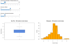
Here’s a link to my Shiny app. This has 4 statistical distributions (normal, lognormal, weibull, exponential) and let’s the user interact with the variables. The box plot and histogram of the data respond to the user controlled inputs.

Check it out here: My Shiny App
(Make sure to give it about 30 seconds to fully load for the first time.)

screenshot

One sample t-test

Perhaps the most widely used statistical analysis for better or worse is the t-test.  Here’s a quick summary of how to call the t-test for one sample using R.  The function name is t.test and the main parameters are the data, the test type (alternative=), the mean (mu=), and the confidence level (conf.level=).

The hardest part about t-tests in R is knowing how to set up the problem.  In these examples the null hypothesis has a mean of 4 (H0: μ = 4) and I have tested the three different alternative hypothesis options: H1: μ ≠ 3, H1: μ < 3, and H1: μ > 3.  In each test I have used a 95% confidence interval (alpha = 0.05).  Note: A t-test would not be performed in this manner using all three alternatives, this is merely for example purposes.

Here’s an example of a one-sided t test using the vector x.

x = c(1,2,4,7,4,3,7,8,3,9)
t.test(x, alternative="two.sided", mu = 3, conf.level = 0.95)
## 
##  One Sample t-test
## 
## data:  x
## t = 2.0769, df = 9, p-value = 0.0676
## alternative hypothesis: true mean is not equal to 3
## 95 percent confidence interval:
##  2.839464 6.760536
## sample estimates:
## mean of x 
##       4.8
t.test(x, alternative="less", mu = 3, conf.level = 0.95)
## 
##  One Sample t-test
## 
## data:  x
## t = 2.0769, df = 9, p-value = 0.9662
## alternative hypothesis: true mean is less than 3
## 95 percent confidence interval:
##      -Inf 6.388698
## sample estimates:
## mean of x 
##       4.8
t.test(x, alternative="greater", mu = 3, conf.level = 0.95)
## 
##  One Sample t-test
## 
## data:  x
## t = 2.0769, df = 9, p-value = 0.0338
## alternative hypothesis: true mean is greater than 3
## 95 percent confidence interval:
##  3.211302      Inf
## sample estimates:
## mean of x 
##       4.8


Let’s analyze the results above starting with the alternative hypothesis that the true mean is not equal to 3 (H1: μ ≠ 3).  The results show that the 95% confidence interval for the true mean is 2.84 to 6.76.  Since the null hypothesis states that the true mean is 3 (H0: μ = 3), and 3 is within the 95% confidence interval, the null hypothesis is unlikely to be rejected.  The p-value is 0.076, which is greater than the alpha value of 0.05 (or 1-confidenc interval 0.95).  Since the p-value is not less than 0.05, the alternative hypothesis that the true mean is not equal to 3 is rejected in favor of the null hypothesis.  Some other useful information the t-test provides is the degrees of freedom (9) and the t-statistic 2.08.

Let’s look at the results from the alternative hypothesis that the true mean is less than 3 (H1: μ < 3).  The 95% confidence interval is less than 6.39 and the p-value is 0.966.  Once again the p-value is greater than the alpha value of 0.05 (or 1-0.95), so the alternative hypothesis that the sample mean is less than 3 (H1: μ < 3) is rejected in favor of the null hypothesis that the true mean is 3 (H0: μ = 3).

Finally let’s look at the results from the t-test using the alternative hypothesis that the true mean is greater than 3 (H1: μ > 3).  The 95% confidence interval is 3.21 and greater, which does not include the value of the null hypothesis.  In this case the p-value is 0.0338, which IS less than the alpha value of 0.05 (or 1-0.95) and the null hypothesis (H0: μ = 3) is rejected in favor of the alternative hypothesis (H1: μ > 3) that the true mean is greater than 3.